The Effective Vertical Anisotropy of Layered Aquifers#
Mark Bakker and Bram Bot.
Notebook to run experiments presented in the paper “The Effective Vertical Anisotropy of Layered Aquifers.”
Reference: M. Bakker and B. Bot (2024) The effective vertical anisotropy of layered aquifers. Groundwater. Available online early: doi.
import matplotlib.pyplot as plt
import numpy as np
from scipy.optimize import brentq

import timml as tml
Function to generate hydraulic conductivities
def generatek(ksection=20 * [0.1, 1], nsections=10, seed=1):
    """Generate k.

    Input:
    ksection: k values in the section
    nsection: number of sections
    seed: seed of random number generator
    """
    nk = len(ksection)
    # nlayers = nk * nsections
    kaq = np.zeros((nsections, nk))
    rng = np.random.default_rng(seed)
    for i in range(nsections):
        kaq[i] = rng.choice(ksection, nk, replace=False)
    return kaq.flatten()
Function to create a model with a canal given kx and kz.
def makemodel(kx, kz, d=4, returnmodel=False):
    """Creates model with river at center, and water supplied from infinitiy.

    d is depth of river.
    """
    H = 40  # thickness of model
    # d = 4 # depth of river
    naq = len(kx)
    ml = tml.Model3D(kaq=kx, z=np.linspace(H, 0, naq + 1), kzoverkh=kz / kx)
    tml.LineSink1D(ml, xls=0, sigls=2, layers=np.arange(int(d * 10)))
    tml.Constant(ml, xr=2000, yr=0, hr=0, layer=0)
    ml.solve(silent=True)
    if returnmodel:
        return ml
    return ml.head(0, 0)[0]


def func(kz, kx, h0, d=4, nlayers=400):
    """Computes head difference."""
    hnew = makemodel(kx * np.ones(nlayers), kz * np.ones(nlayers), d, returnmodel=False)
    return hnew - h0
Function to create a model with a partially penetrating well.
def makemodelradial(kx, kz, d=4, rw=0.1, returnmodel=False):
    """Creates model with river at center, and water supplied from infinitiy."""
    H = 40  # thickness of model
    # d = 4 # depth of river
    Qw = 1000
    naq = len(kx)
    ml = tml.Model3D(kaq=kx, z=np.linspace(H, 0, naq + 1), kzoverkh=kz / kx)
    tml.Well(ml, xw=0, yw=0, Qw=Qw, rw=rw, layers=np.arange(int(d * 10)))
    tml.Constant(ml, xr=2000, yr=0, hr=0, layer=0)
    ml.solve(silent=True)
    if returnmodel:
        return ml
    return ml.head(0, 0)[0]


def funcradial(kz, kx, h0, d=4, rw=0.1, nlayers=400):
    """Computes head difference."""
    hnew = makemodelradial(
        kx * np.ones(nlayers), kz * np.ones(nlayers), d, rw, returnmodel=False
    )
    return hnew - h0
Find effective vertical hydraulic conductivity for one realization of 400 layers and time it
kaq = 80 * [1, 3.16, 10, 31.6, 100]  # 400 k values
k = generatek(ksection=kaq, nsections=1)  # random order of k values
h0 = makemodel(k, k)  # head at canal
kx = np.mean(k)  # equivalent horizontal k
# vertical hydraulic conductivity:
%timeit kz = brentq(func, a=0.001 * kx, b=kx, args=(kx, h0))
3.11 s ± 24.3 ms per loop (mean ± std. dev. of 7 runs, 1 loop each)
Run the experiment for Figure 3a. This is commented out because it takes a long time to run. The number of the realization is printed to the screen every 10 realizations.
So 1000 realizations takes on the order of 3000 seconds (on this machine), so around 50 minutes.
kaq = np.array(80 * [1, 3.16, 10, 31.6, 100])
ntot = 1000
aniso = np.zeros(ntot)

for i in range(ntot):
    k = generatek(kaq, nsections=1, seed=i)
    h0 = makemodel(k, k)
    kx = np.mean(k)
    kz = brentq(func, a=0.001 * kx, b=kx, args=(kx, h0))
    aniso[i] = kx / kz
    if i % 10 == 0:
        print(i, end=" ")
print("\n completed")
0
---------------------------------------------------------------------------
KeyboardInterrupt                         Traceback (most recent call last)
Cell In[6], line 9
      7 h0 = makemodel(k, k)
      8 kx = np.mean(k)
----> 9 kz = brentq(func, a=0.001 * kx, b=kx, args=(kx, h0))
     10 aniso[i] = kx / kz
     11 if i % 10 == 0:

File ~/checkouts/readthedocs.org/user_builds/timml/envs/latest/lib/python3.11/site-packages/scipy/optimize/_zeros_py.py:846, in brentq(f, a, b, args, xtol, rtol, maxiter, full_output, disp)
    844     raise ValueError(f"rtol too small ({rtol:g} < {_rtol:g})")
    845 f = _wrap_nan_raise(f)
--> 846 r = _zeros._brentq(f, a, b, xtol, rtol, maxiter, args, full_output, disp)
    847 return results_c(full_output, r, "brentq")

File ~/checkouts/readthedocs.org/user_builds/timml/envs/latest/lib/python3.11/site-packages/scipy/optimize/_zeros_py.py:94, in _wrap_nan_raise.<locals>.f_raise(x, *args)
     93 def f_raise(x, *args):
---> 94     fx = f(x, *args)
     95     f_raise._function_calls += 1
     96     if np.isnan(fx):

Cell In[3], line 20, in func(kz, kx, h0, d, nlayers)
     18 def func(kz, kx, h0, d=4, nlayers=400):
     19     """Computes head difference."""
---> 20     hnew = makemodel(kx * np.ones(nlayers), kz * np.ones(nlayers), d, returnmodel=False)
     21     return hnew - h0

Cell In[3], line 12, in makemodel(kx, kz, d, returnmodel)
     10 tml.LineSink1D(ml, xls=0, sigls=2, layers=np.arange(int(d * 10)))
     11 tml.Constant(ml, xr=2000, yr=0, hr=0, layer=0)
---> 12 ml.solve(silent=True)
     13 if returnmodel:
     14     return ml

File ~/checkouts/readthedocs.org/user_builds/timml/envs/latest/lib/python3.11/site-packages/timml/model.py:455, in Model.solve(self, printmat, sendback, silent)
    450 for e in self.elementlist:
    451     if e.nunknowns > 0:
    452         (
    453             mat[ieq : ieq + e.nunknowns, :],
    454             rhs[ieq : ieq + e.nunknowns],
--> 455         ) = e.equation()
    456         ieq += e.nunknowns
    457     if silent is False:

File ~/checkouts/readthedocs.org/user_builds/timml/envs/latest/lib/python3.11/site-packages/timml/equation.py:165, in MscreenWellEquation.equation(self)
    162 for e in self.model.elementlist:
    163     if e.nunknowns > 0:
    164         head = (
--> 165             e.potinflayers(self.xc[0], self.yc[0], self.layers)
    166             / self.aq.Tcol[self.layers, :]
    167         )
    168         mat[0 : self.nlayers - 1, ieq : ieq + e.nunknowns] = head[:-1] - head[1:]
    169         if e == self:

File ~/checkouts/readthedocs.org/user_builds/timml/envs/latest/lib/python3.11/site-packages/timml/element.py:63, in Element.potinflayers(self, x, y, layers, aq)
     61     aq = self.model.aq.find_aquifer_data(x, y)
     62 pot = self.potinf(x, y, aq)  # nparam rows, naq cols
---> 63 rv = np.sum(
     64     pot[:, np.newaxis, :] * aq.eigvec, 2
     65 ).T  # Transopose as the first axes needs to be the number of layers
     66 return rv[layers, :]

File ~/checkouts/readthedocs.org/user_builds/timml/envs/latest/lib/python3.11/site-packages/numpy/_core/fromnumeric.py:2333, in _sum_dispatcher(a, axis, dtype, out, keepdims, initial, where)
   2327         raise ValueError("Passing `min` or `max` keyword argument when "
   2328                          "`a_min` and `a_max` are provided is forbidden.")
   2330     return _wrapfunc(a, 'clip', a_min, a_max, out=out, **kwargs)
-> 2333 def _sum_dispatcher(a, axis=None, dtype=None, out=None, keepdims=None,
   2334                     initial=None, where=None):
   2335     return (a, out)
   2338 @array_function_dispatch(_sum_dispatcher)
   2339 def sum(a, axis=None, dtype=None, out=None, keepdims=np._NoValue,
   2340         initial=np._NoValue, where=np._NoValue):

KeyboardInterrupt:
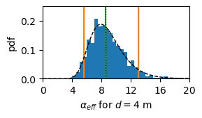
Create figure 3a
from scipy.stats import lognorm


def create_fig3a():
    plt.figure(figsize=(3, 3))
    plt.subplot(211)
    plt.hist(aniso, bins=np.arange(2, 20, 0.5), density=True)
    p5, p50, p95 = np.percentile(aniso, [5, 50, 95])
    # print('p5, p50, p95', p5, p50, p95)
    plt.axvline(p5, color="C1")
    plt.axvline(p95, color="C1")
    plt.axvline(p50, color="C2")
    kheq = np.mean(kaq)
    kveq = len(kaq) / np.sum(1 / kaq)
    anisoeq = kheq / kveq
    plt.axvline(anisoeq, color="k", linestyle=":", linewidth=1)
    #
    shape, loc, scale = lognorm.fit(aniso)
    # print('shape, loc, scale: ', shape, loc, scale)
    x = np.linspace(0, 20, 100)
    pdf1 = lognorm.pdf(x, shape, loc, scale)
    plt.plot(x, pdf1, "k--", lw=1)
    plt.xlim(0, 20)
    plt.ylim(0, 0.25)
    plt.xticks(np.arange(0, 21, 4))
    plt.xlabel(r"$\alpha_{eff}$ for $d=4$ m")
    plt.ylabel("pdf")
    plt.tight_layout()
# Only run if anisotropy has been computed
create_fig3a()