A well in uniform flow

Consider a well in the middle aquifer of a three aquifer system. Aquifer properties are given in Table 1. The well is located at \((x,y)=(0,0)\), the discharge is \(Q=10,000\) m\(^3\)/d and the radius is 0.2 m. There is a uniform flow from West to East with a gradient of 0.002. The head is fixed to 20 m at a distance of 10,000 m downstream of the well. Here is the cookbook recipe to build this model:

• Import numpy: import numpy as np

• Import pyplot for plotting: import matplotlib.pyplot as plt

• Import TimML: import timml as tml

• Create the model and give it a name, for example ml with the command ml = tml.ModelMaq(kaq, z, c) (substitute the correct lists for kaq, z, and c).

• Enter the well with the command w = tml.Well(ml, xw, yw, Qw, rw, layers), where the well is called w.

• Enter uniform flow with the command tml.Uflow(ml, slope, angle).

• Enter the reference head with tml.Constant(ml, xr, yr, head, layer).

• Solve the model ml.solve()

Table 1: Aquifer data for exercise 1

Layer	\(k\) (m/d)	\(z_b\) (m)	\(z_t\)	\(c\) (days)
Aquifer 0	10	-20	0	-
Leaky Layer 1	-	-40	-20	4000
Aquifer 1	20	-80	-40	-
Leaky Layer 2	-	-90	-80	10000
Aquifer 2	5	-140	-90	-

import numpy as np

import timml as tml

figsize = (8, 8)

ml = tml.ModelMaq(kaq=[10, 20, 5], z=[0, -20, -40, -80, -90, -140], c=[4000, 10000])
w = tml.Well(ml, xw=0, yw=0, Qw=10000, rw=0.2, layers=1)
tml.Constant(ml, xr=10000, yr=0, hr=20, layer=0)
tml.Uflow(ml, slope=0.002, angle=0)
ml.solve()

Number of elements, Number of equations: 3 , 1
.
.
.

solution complete

Questions:

Exercise 1a

What are the leakage factors of the aquifer system?

print("The leakage factors of the aquifers are:")
print(ml.aq.lab)

The leakage factors of the aquifers are:
[   0.         1430.58042146  790.84743012]

Exercise 1b

What is the head at the well?

print("The head at the well is:")
print(w.headinside())

The head at the well is:
[20.06196743]

Exercise 1c

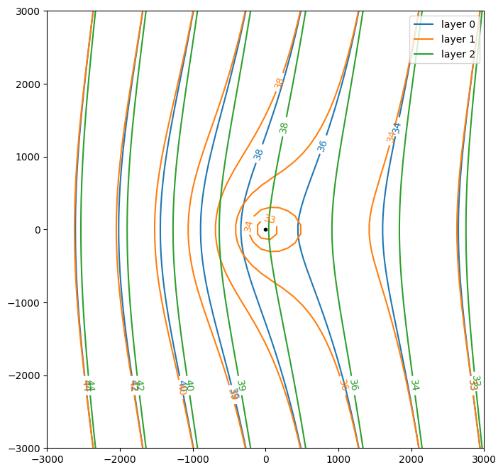
Create a contour plot of the head in the three aquifers. Use a window with lower left hand corner \((x,y)=(−3000,−3000)\) and upper right hand corner \((x,y)=(3000,3000)\). Notice that the heads in the three aquifers are almost equal at three times the largest leakage factor.

ml.plots.contour(
    win=[-3000, 3000, -3000, 3000],
    ngr=50,
    layers=[0, 1, 2],
    levels=10,
    legend=True,
    figsize=figsize,
)

[<matplotlib.contour.QuadContourSet at 0x79d2c5a85a90>,
 <matplotlib.contour.QuadContourSet at 0x79d2c5aa6790>,
 <matplotlib.contour.QuadContourSet at 0x79d2c5aafb90>]

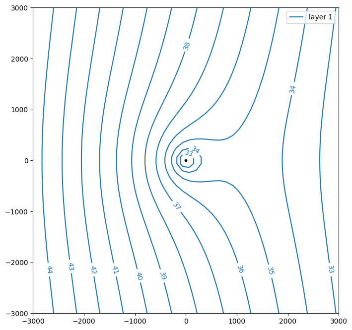
Exercise 1d

Create a contour plot of the head in aquifer 1 with labels along the contours. Labels are added when the labels keyword argument is set to True. The number of decimal places can be set with the decimals keyword argument, which is zero by default.

ml.plots.contour(
    win=[-3000, 3000, -3000, 3000],
    ngr=50,
    layers=[1],
    levels=np.arange(30, 45, 1),
    labels=True,
    legend=["layer 1"],
    figsize=figsize,
)

[<matplotlib.contour.QuadContourSet at 0x79d2c56cadd0>]

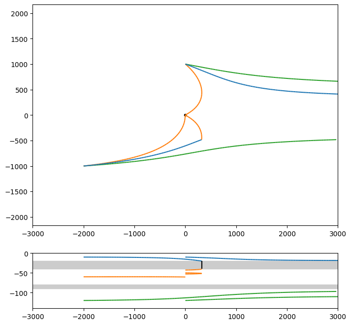
Exercise 1e

Create a contour plot with a vertical cross-section below it. Start three pathlines from \((x,y)=(-2000,-1000)\) at levels \(z=-120\), \(z=-60\), and \(z=-10\). Try a few other starting locations.

win = [-3000, 3000, -3000, 3000]
ml.plots.topview(win=win, orientation="both", figsize=figsize)
ml.plots.tracelines(
    -2000 * np.ones(3),
    -1000 * np.ones(3),
    [-120, -60, -10],
    hstepmax=50,
    win=win,
    orientation="both",
)
ml.plots.tracelines(
    0 * np.ones(3),
    1000 * np.ones(3),
    [-120, -50, -10],
    hstepmax=50,
    win=win,
    orientation="both",
)

.
.
.

.
.
.

Ignoring fixed y limits to fulfill fixed data aspect with adjustable data limits.

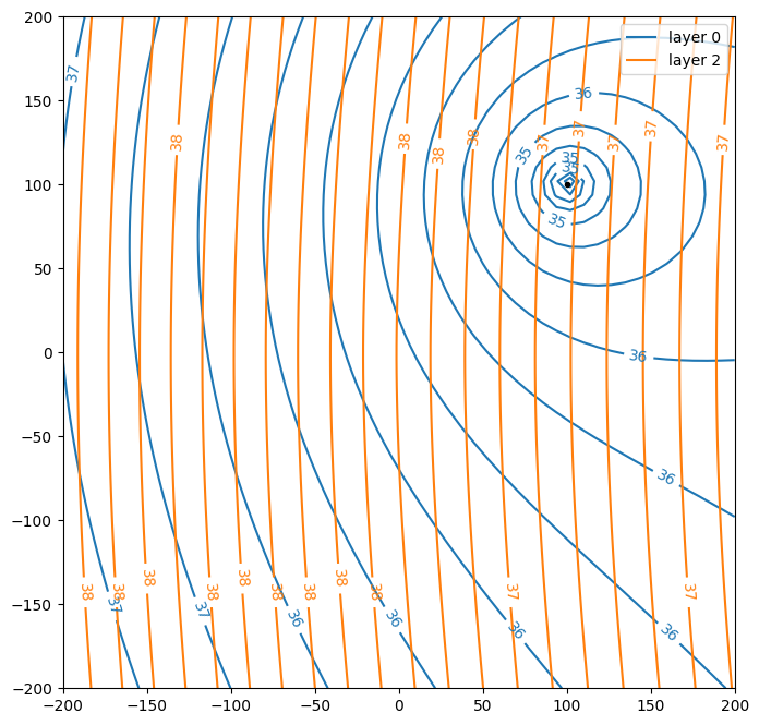
Exercise 1f

Add an abandoned well that is screened in both aquifer 0 and aquifer 1, located at \((x, y) = (100, 100)\) and create contour plot of all aquifers near the well (from (-200,-200) till (200,200)). What are the discharge and the head at the abandoned well? Note that you have to solve the model again!

ml = tml.ModelMaq(kaq=[10, 20, 5], z=[0, -20, -40, -80, -90, -140], c=[4000, 10000])
w = tml.Well(ml, xw=0, yw=0, Qw=10000, rw=0.2, layers=1)
tml.Constant(ml, xr=10000, yr=0, hr=20, layer=0)
tml.Uflow(ml, slope=0.002, angle=0)
wabandoned = tml.Well(ml, xw=100, yw=100, Qw=0, rw=0.2, layers=[0, 1])
ml.solve()
ml.plots.contour(
    win=[-200, 200, -200, 200],
    ngr=50,
    layers=[0, 2],
    levels=20,
    color=["C0", "C1", "C2"],
    legend=True,
    figsize=figsize,
)

Number of elements, Number of equations: 4 , 3
.
.
.
.

solution complete

[<matplotlib.contour.QuadContourSet at 0x79d2c57ef550>,
 <matplotlib.contour.QuadContourSet at 0x79d2c57d3e10>]

print("The head at the abandoned well is:")
print(wabandoned.headinside())
print("The discharge at the abandoned well is:")
print(wabandoned.discharge())

The head at the abandoned well is:
[33.62101294 33.62101294]
The discharge at the abandoned well is:
[ 431.40914098 -431.40914098    0.        ]