The Effective Vertical Anisotropy of Layered Aquifers#
Mark Bakker and Bram Bot.
Notebook to run experiments presented in the paper “The Effective Vertical Anisotropy of Layered Aquifers.”
Reference: M. Bakker and B. Bot (2024) The effective vertical anisotropy of layered aquifers. Groundwater. Available online early: doi.
import matplotlib.pyplot as plt
import numpy as np
from scipy.optimize import brentq

import timml as tml
Function to generate hydraulic conductivities
def generatek(ksection=20 * [0.1, 1], nsections=10, seed=1):
    """Generate k.

    Input:
    ksection: k values in the section
    nsection: number of sections
    seed: seed of random number generator
    """
    nk = len(ksection)
    # nlayers = nk * nsections
    kaq = np.zeros((nsections, nk))
    rng = np.random.default_rng(seed)
    for i in range(nsections):
        kaq[i] = rng.choice(ksection, nk, replace=False)
    return kaq.flatten()
Function to create a model with a canal given kx and kz.
def makemodel(kx, kz, d=4, returnmodel=False):
    """Creates model with river at center, and water supplied from infinitiy.

    d is depth of river.
    """
    H = 40  # thickness of model
    # d = 4 # depth of river
    naq = len(kx)
    ml = tml.Model3D(kaq=kx, z=np.linspace(H, 0, naq + 1), kzoverkh=kz / kx)
    tml.LineSink1D(ml, xls=0, sigls=2, layers=np.arange(int(d * 10)))
    tml.Constant(ml, xr=2000, yr=0, hr=0, layer=0)
    ml.solve(silent=True)
    if returnmodel:
        return ml
    return ml.head(0, 0)[0]


def func(kz, kx, h0, d=4, nlayers=400):
    """Computes head difference."""
    hnew = makemodel(kx * np.ones(nlayers), kz * np.ones(nlayers), d, returnmodel=False)
    return hnew - h0
Function to create a model with a partially penetrating well.
def makemodelradial(kx, kz, d=4, rw=0.1, returnmodel=False):
    """Creates model with river at center, and water supplied from infinitiy."""
    H = 40  # thickness of model
    # d = 4 # depth of river
    Qw = 1000
    naq = len(kx)
    ml = tml.Model3D(kaq=kx, z=np.linspace(H, 0, naq + 1), kzoverkh=kz / kx)
    tml.Well(ml, xw=0, yw=0, Qw=Qw, rw=rw, layers=np.arange(int(d * 10)))
    tml.Constant(ml, xr=2000, yr=0, hr=0, layer=0)
    ml.solve(silent=True)
    if returnmodel:
        return ml
    return ml.head(0, 0)[0]


def funcradial(kz, kx, h0, d=4, rw=0.1, nlayers=400):
    """Computes head difference."""
    hnew = makemodelradial(
        kx * np.ones(nlayers), kz * np.ones(nlayers), d, rw, returnmodel=False
    )
    return hnew - h0
Find effective vertical hydraulic conductivity for one realization of 400 layers and time it
kaq = 80 * [1, 3.16, 10, 31.6, 100]  # 400 k values
k = generatek(ksection=kaq, nsections=1)  # random order of k values
h0 = makemodel(k, k)  # head at canal
kx = np.mean(k)  # equivalent horizontal k
# vertical hydraulic conductivity:
%timeit kz = brentq(func, a=0.001 * kx, b=kx, args=(kx, h0))
2.35 s ± 6.71 ms per loop (mean ± std. dev. of 7 runs, 1 loop each)
Run the experiment for Figure 3a. This is commented out because it takes a long time to run. The number of the realization is printed to the screen every 10 realizations.
So 1000 realizations takes on the order of 3000 seconds (on this machine), so around 50 minutes.
kaq = np.array(80 * [1, 3.16, 10, 31.6, 100])
ntot = 1000
aniso = np.zeros(ntot)

for i in range(ntot):
    k = generatek(kaq, nsections=1, seed=i)
    h0 = makemodel(k, k)
    kx = np.mean(k)
    kz = brentq(func, a=0.001 * kx, b=kx, args=(kx, h0))
    aniso[i] = kx / kz
    if i % 10 == 0:
        print(i, end=" ")
print("\n completed")
0
10
---------------------------------------------------------------------------
KeyboardInterrupt                         Traceback (most recent call last)
Cell In[6], line 9
      7 h0 = makemodel(k, k)
      8 kx = np.mean(k)
----> 9 kz = brentq(func, a=0.001 * kx, b=kx, args=(kx, h0))
     10 aniso[i] = kx / kz
     11 if i % 10 == 0:

File ~/checkouts/readthedocs.org/user_builds/timml/envs/stable/lib/python3.11/site-packages/scipy/optimize/_zeros_py.py:846, in brentq(f, a, b, args, xtol, rtol, maxiter, full_output, disp)
    844     raise ValueError(f"rtol too small ({rtol:g} < {_rtol:g})")
    845 f = _wrap_nan_raise(f)
--> 846 r = _zeros._brentq(f, a, b, xtol, rtol, maxiter, args, full_output, disp)
    847 return results_c(full_output, r, "brentq")

File ~/checkouts/readthedocs.org/user_builds/timml/envs/stable/lib/python3.11/site-packages/scipy/optimize/_zeros_py.py:94, in _wrap_nan_raise.<locals>.f_raise(x, *args)
     93 def f_raise(x, *args):
---> 94     fx = f(x, *args)
     95     f_raise._function_calls += 1
     96     if np.isnan(fx):

Cell In[3], line 20, in func(kz, kx, h0, d, nlayers)
     18 def func(kz, kx, h0, d=4, nlayers=400):
     19     """Computes head difference."""
---> 20     hnew = makemodel(kx * np.ones(nlayers), kz * np.ones(nlayers), d, returnmodel=False)
     21     return hnew - h0

Cell In[3], line 12, in makemodel(kx, kz, d, returnmodel)
     10 tml.LineSink1D(ml, xls=0, sigls=2, layers=np.arange(int(d * 10)))
     11 tml.Constant(ml, xr=2000, yr=0, hr=0, layer=0)
---> 12 ml.solve(silent=True)
     13 if returnmodel:
     14     return ml

File ~/checkouts/readthedocs.org/user_builds/timml/envs/stable/lib/python3.11/site-packages/timml/model.py:433, in Model.solve(self, printmat, sendback, silent)
    431 """Compute solution."""
    432 # Initialize elements
--> 433 self.initialize()
    434 # Compute number of equations
    435 self.neq = np.sum([e.nunknowns for e in self.elementlist])

File ~/checkouts/readthedocs.org/user_builds/timml/envs/stable/lib/python3.11/site-packages/timml/model.py:72, in Model.initialize(self)
     69 def initialize(self):
     70     # remove inhomogeneity elements (they are added again)
     71     self.elementlist = [e for e in self.elementlist if not e.inhomelement]
---> 72     self.aq.initialize()
     73     for e in self.elementlist:
     74         e.initialize()

File ~/checkouts/readthedocs.org/user_builds/timml/envs/stable/lib/python3.11/site-packages/timml/aquifer.py:197, in Aquifer.initialize(self)
    195 def initialize(self):
    196     # cause we are going to call initialize for inhoms
--> 197     AquiferData.initialize(self)
    198     for inhom in self.inhomlist:
    199         inhom.initialize()

File ~/checkouts/readthedocs.org/user_builds/timml/envs/stable/lib/python3.11/site-packages/timml/aquifer.py:94, in AquiferData.initialize(self)
     92 dm1 = -1.0 / (self.c[1:] * self.T[:-1])
     93 A = np.diag(dm1, -1) + np.diag(d0, 0) + np.diag(dp1, 1)
---> 94 w, v = np.linalg.eig(A)
     95 # take the real part for the rare occasion that the eig
     96 # function returns a complex answer with very small
     97 # imaginary part
     98 w = w.real

File ~/checkouts/readthedocs.org/user_builds/timml/envs/stable/lib/python3.11/site-packages/numpy/linalg/_linalg.py:1523, in eig(a)
   1519 signature = 'D->DD' if isComplexType(t) else 'd->DD'
   1520 with errstate(call=_raise_linalgerror_eigenvalues_nonconvergence,
   1521               invalid='call', over='ignore', divide='ignore',
   1522               under='ignore'):
-> 1523     w, vt = _umath_linalg.eig(a, signature=signature)
   1525 if not isComplexType(t) and all(w.imag == 0.0):
   1526     w = w.real

KeyboardInterrupt:
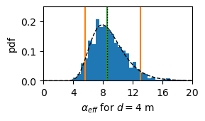
Create figure 3a
from scipy.stats import lognorm


def create_fig3a():
    plt.figure(figsize=(3, 3))
    plt.subplot(211)
    plt.hist(aniso, bins=np.arange(2, 20, 0.5), density=True)
    p5, p50, p95 = np.percentile(aniso, [5, 50, 95])
    # print('p5, p50, p95', p5, p50, p95)
    plt.axvline(p5, color="C1")
    plt.axvline(p95, color="C1")
    plt.axvline(p50, color="C2")
    kheq = np.mean(kaq)
    kveq = len(kaq) / np.sum(1 / kaq)
    anisoeq = kheq / kveq
    plt.axvline(anisoeq, color="k", linestyle=":", linewidth=1)
    #
    shape, loc, scale = lognorm.fit(aniso)
    # print('shape, loc, scale: ', shape, loc, scale)
    x = np.linspace(0, 20, 100)
    pdf1 = lognorm.pdf(x, shape, loc, scale)
    plt.plot(x, pdf1, "k--", lw=1)
    plt.xlim(0, 20)
    plt.ylim(0, 0.25)
    plt.xticks(np.arange(0, 21, 4))
    plt.xlabel(r"$\alpha_{eff}$ for $d=4$ m")
    plt.ylabel("pdf")
    plt.tight_layout()
# Only run if anisotropy has been computed
create_fig3a()