Recharge in a circular area

This notebook demonstrates how to model a circular area with constant recharge or extraction using the CircAreaSink element.

import matplotlib.pyplot as plt
import numpy as np

import timml as tml

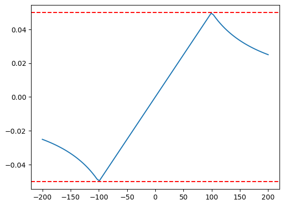
Circular area-sink with radius 100 m, located at the origin.

N = 0.001
R = 100
ml = tml.ModelMaq(kaq=5, z=[10, 0])
ca = tml.CircAreaSink(ml, xc=0, yc=0, R=100, N=0.001)
ml.solve()
x = np.linspace(-200, 200, 100)
h = ml.headalongline(x, 0)
plt.plot(x, h[0]);

Number of elements, Number of equations: 1 , 0
No unknowns. Solution complete

qx = np.zeros_like(x)
for i in range(len(x)):
    qx[i], qy = ml.disvec(x[i], 1e-6)
plt.plot(x, qx)
qxb = N * np.pi * R**2 / (2 * np.pi * R)
plt.axhline(qxb, color="r", ls="--")
plt.axhline(-qxb, color="r", ls="--");

/tmp/ipykernel_897/4090603064.py:3: DeprecationWarning: Conversion of an array with ndim > 0 to a scalar is deprecated, and will error in future. Ensure you extract a single element from your array before performing this operation. (Deprecated NumPy 1.25.)
  qx[i], qy = ml.disvec(x[i], 1e-6)

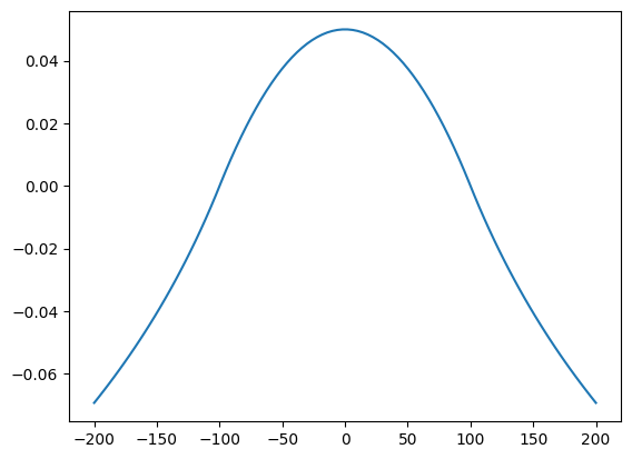
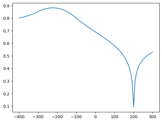
Circular area-sink and well

Discharge of well is the same as total infiltration rate of the circular area-sink. Well and center of area-sink area located at equal distances from \(y\)-axis, so that the head remains zero along the \(y\)-axis. Solution approaches steady-state solution.

N = 0.001
R = 100
Q = N * np.pi * R**2
ml = tml.ModelMaq(kaq=5, z=[10, 0])
ca = tml.CircAreaSink(ml, xc=-200, yc=0, R=100, N=0.001)
w = tml.Well(ml, 200, 0, Qw=Q, rw=0.1)
ml.solve()
x = np.linspace(-400, 300, 100)
h = ml.headalongline(x, 0)
plt.plot(x, h[0]);

Number of elements, Number of equations: 2 , 0
No unknowns. Solution complete

N = 0.001
R = 100
Q = N * np.pi * R**2
ml = tml.ModelMaq(kaq=5, z=[10, 0])
ca = tml.CircAreaSink(ml, xc=-200, yc=0, R=100, N=0.001)
w = tml.Well(ml, 200, 0, Qw=Q, rw=0.1)
ml.solve()
ml.plots.contour([-300, 300, -200, 200], ngr=40)

Number of elements, Number of equations: 2 , 0
No unknowns. Solution complete

[<matplotlib.contour.QuadContourSet at 0x73346d516450>]

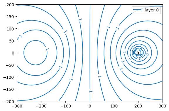
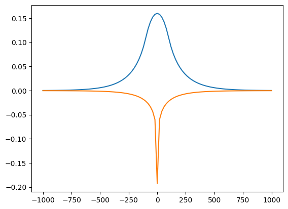
Two layers

Discharge of well is the same as total infiltration rate of the circular area-sink. Center of area-sink and well are at the origin. Circular area-sink in layer 0, well in layer 1.

N = 0.001
R = 100
Q = N * np.pi * R**2
ml = tml.ModelMaq(kaq=[5, 20], z=[20, 12, 10, 0], c=[1000])
ca = tml.CircAreaSink(ml, xc=0, yc=0, R=100, N=0.001)
w = tml.Well(ml, 0, 0, Qw=Q, rw=0.1, layers=1)
rf = tml.Constant(ml, 1000, 0, 0)
ml.solve()
x = np.linspace(-200, 200, 100)
h = ml.headalongline(x, 0)
plt.plot(x, h[0])
plt.plot(x, h[1]);

Number of elements, Number of equations: 3 , 1
.
.
.

solution complete

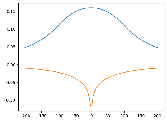
x = np.linspace(-1000, 1000, 101)
h = ml.headalongline(x, 0)
plt.plot(x, h[0])
plt.plot(x, h[1]);