Horizontal wells#
A horizontal well is located in a 20 m thick aquifer; the hydraulic conductivity is \(k = 10\) m/d and the vertical anisotropy factor is 0.1. The horizontal well is placed 5 m above the bottom of the aquifer. The well has a discharge of 10,000 m\(^3\)/d and radius of \(r=0.2\) m. The well is 200 m long and runs from \((x, y) = (−100, 0)\) to \((x, y) = (100, 0)\). A long straight river with a head of 40 m runs to the right of the horizontal well along the line \(x = 200\). The head is fixed to 42 m at \((x, y) = (−1000, 0)\).
Three-dimensional flow to the horizontal well is modeled by dividing the aquifer up in 11 layers; the
elevations are: [20, 15, 10, 8, 6, 5.5, 5.2, 4.8, 4.4, 4, 2, 0]. At the depth of the well, the layer thickness is equal to
the diameter of the well, and it increases in the layers above and below the well. A TimML model is created with the Model3D
command. The horizontal well is located in layer 6 and is modeled with the Ditch element. Initially, the entry resistance of the well is set to zero.
import matplotlib.pyplot as plt
import numpy as np

import timml as tml

figsize = (8, 8)
z = [20, 15, 10, 8, 6, 5.5, 5.2, 4.8, 4.4, 4, 2, 0]
ml = tml.Model3D(kaq=10, z=z, kzoverkh=0.1)
ls1 = tml.Ditch(ml, x1=-100, y1=0, x2=100, y2=0, Qls=10000, order=5, layers=6)
ls2 = tml.RiverString(
    ml,
    [(200, -1000), (200, -200), (200, 0), (200, 200), (200, 1000)],
    hls=40,
    order=5,
    layers=0,
)
rf = tml.Constant(ml, xr=-1000, yr=0, hr=42, layer=0)
Questions:#
Exercise 4a#
Solve the model.
ml.solve()
Number of elements, Number of equations: 3 , 31
.
.
.

solution complete
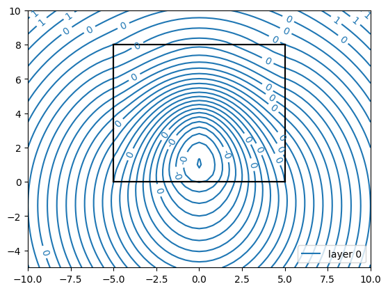
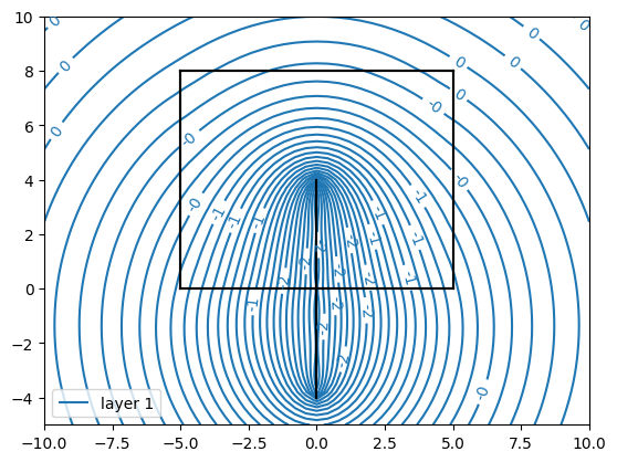
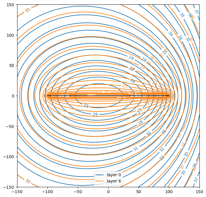
Exercise 4b#
Create contour plots of layers 0 and 6 and note the difference between the layers. Also, compute the head at \((x, y) = (0, 0.2)\) (on the edge of the well) and notice that there is a very large head difference between the top of the aquifer and the well.
ml.plots.contour(
    win=[-150, 150, -150, 150], ngr=[50, 100], layers=[0, 6], figsize=figsize
)
print("The head at the top and in layer 6 are:")
print(ml.head(0, 0.2, [0, 6]))
The head at the top and in layer 6 are:
[24.75850319 13.05654353]
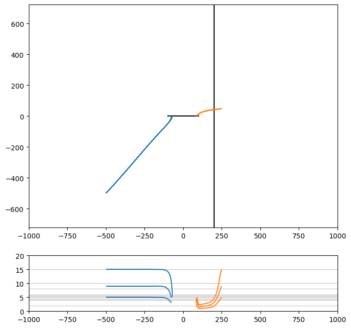
Exercise 4c#
Draw a number of pathlines from different elevations using the tracelines command. First make a plot with a cross section below it.
ml.plots.topview(win=[-1000, 1000, -1000, 1000], orientation="both", figsize=figsize)
ml.plots.tracelines(
    xstart=[-500, -500, -500],
    ystart=[-500, -500, -500],
    zstart=[5, 9, 15],
    hstepmax=20,
    tmax=10 * 365.25,
    orientation="both",
    color="C0",
)
ml.plots.tracelines(
    xstart=[250, 250, 250],
    ystart=[50, 50, 50],
    zstart=[5, 9, 15],
    hstepmax=20,
    tmax=10 * 365.25,
    orientation="both",
    color="C1",
)
.
.
.

.
.
.
Ignoring fixed y limits to fulfill fixed data aspect with adjustable data limits.
Exercise 4d#
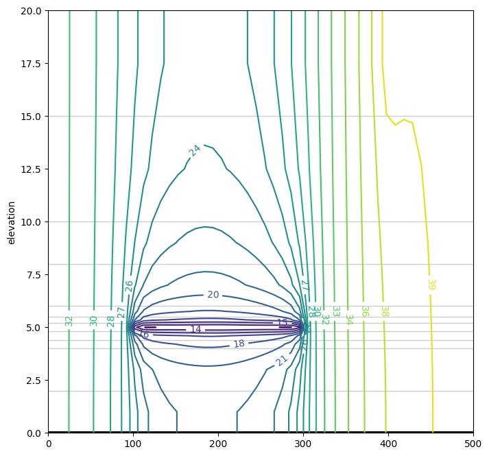
Make a contour plot of the heads in a vertical cross-section using the vcontour command. Use a cross-section along the well.
ml.plots.vcontour(win=[-200, 300, 0, 0], n=50, levels=20, figsize=figsize)
<matplotlib.contour.QuadContourSet at 0x7f8f2e8b3690>
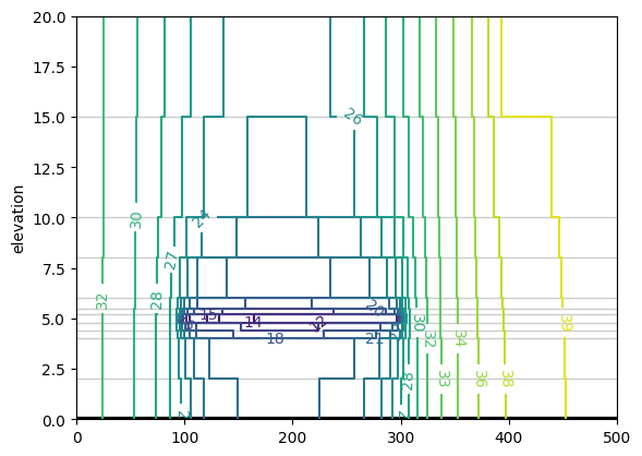
Exercise 4e#
Change the entry resistance of the horizontal well to 0.01 days and set the width to 0.4 m and resolve the model. Notice the difference in the head inside the horizontal well with the headinside function of the horizontal well. Use a
print("head inside w/o resistance:")
print(ls1.headinside())
head inside w/o resistance:
[12.1087613]
ml = tml.Model3D(kaq=10, z=z, kzoverkh=0.1)
ls = tml.Ditch(
    ml, x1=-100, y1=0, x2=100, y2=0, Qls=10000, order=5, layers=6, wh=0.4, res=0.01
)
tml.RiverString(
    ml,
    [(200, -1000), (200, -200), (200, 0), (200, 200), (200, 1000)],
    hls=40,
    order=5,
    layers=0,
)
rf = tml.Constant(ml, xr=-1000, yr=0, hr=42, layer=0)
ml.solve()
Number of elements, Number of equations: 3 , 31
.
.
.

solution complete
print("head inside horizontal well:", ls.headinside())
head inside horizontal well: [10.83630693]
ml.plots.vcontour(win=[-200, 300, 0, 0], n=50, levels=20, vinterp=False)
<matplotlib.contour.QuadContourSet at 0x7f8f2efe3950>
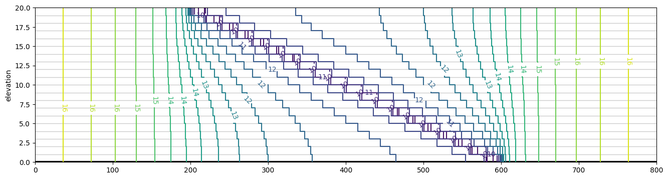
Slanted well#
A slanted well may be simulated by putting different sections in different layers
z = [20, 15, 10, 8, 6, 5.5, 5.2, 4.8, 4.4, 4, 2, 0]
ml = tml.Model3D(kaq=10, z=np.linspace(20, 0, 21), kzoverkh=0.1)
rf = tml.Constant(ml, 0, 1000, 20)
x = np.linspace(-200, 200, 21)
y = np.zeros(21)
ls = tml.RiverString(
    ml, xy=list(zip(x, y, strict=False)), hls=10, layers=np.arange(0, 20, 1), order=0
)
ml.solve()
Number of elements, Number of equations: 2 , 21
.
.

solution complete
ml.plots.vcontour(win=[-400, 400, 0, 0], n=200, levels=20, vinterp=False, figsize=(16, 4))
<matplotlib.contour.QuadContourSet at 0x7f8f2ec20310>

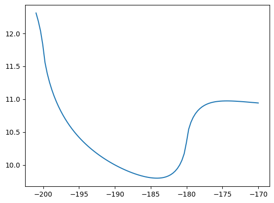
Note that the head is not exactly constant along the line-sink segments when using order 0
h = ml.headalongline(np.linspace(-201, -170, 100), 0)
plt.plot(np.linspace(-201, -170, 100), h[0])
[<matplotlib.lines.Line2D at 0x7f8f2f4ffc90>]
Qtot = np.sum(ls.discharge())
print("Discharge of slanted well when modeled with fixed head hls=10:", Qtot)
Discharge of slanted well when modeled with fixed head hls=10: 4193.946003637198
z = [20, 15, 10, 8, 6, 5.5, 5.2, 4.8, 4.4, 4, 2, 0]
ml = tml.Model3D(kaq=10, z=np.linspace(20, 0, 21), kzoverkh=0.1)
rf = tml.Constant(ml, 0, 1000, 20)
x = np.linspace(-200, 200, 21)
y = np.zeros(21)
ls = tml.DitchString(
    ml, xy=list(zip(x, y, strict=False)), Qls=Qtot, layers=np.arange(0, 20, 1), order=0
)
ml.solve()
Number of elements, Number of equations: 2 , 21
.
.

solution complete
ml.plots.vcontour(win=[-400, 400, 0, 0], n=200, levels=20, vinterp=False, figsize=(16, 4))
<matplotlib.contour.QuadContourSet at 0x7f8f2f3f38d0>
print("Head in slanted well when modeled with fixed discharge:")
[print(lspart.headinside()) for lspart in ls.lslist];
Head in slanted well when modeled with fixed discharge:
[10.]
[10.]
[10.]
[10.]
[10.]
[10.]
[10.]
[10.]
[10.]
[10.]
[10.]
[10.]
[10.]
[10.]
[10.]
[10.]
[10.]
[10.]
[10.]
[10.]
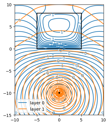
Lake with a horizontal well#
import timml as tml
ml = tml.ModelMaq(kaq=[1, 2], z=[10, 5, 4, 0], c=20)
xy = [(-5, 0), (0, 0), (5, 0), (5, 8), (-5, 8)]
p1 = tml.PolygonInhomMaq(
    ml,
    xy=xy,
    kaq=[0.2, 8],
    z=[11, 10, 5, 4, 0],
    c=[2, 20],
    topboundary="semi",
    hstar=1.0,
    order=3,
    ndeg=1,
)
w = tml.Well(ml, xw=0, yw=-10, Qw=100, layers=1)
rf = tml.Constant(ml, xr=0, yr=-100, hr=2)
ml.solve()

ml.plots.contour([-10, 10, -15, 10], 50, [0, 1], 30)
Number of elements, Number of equations: 13 , 81
.
.
.
.
.
.
.
.
.
.
.
.
.

solution complete
[<matplotlib.contour.QuadContourSet at 0x7f8f2f25c350>,
 <matplotlib.contour.QuadContourSet at 0x7f8f2f314950>]
ml = tml.ModelMaq(kaq=[1, 2], z=[10, 5, 4, 0], c=20)
xy = [(-5, 0), (0, 0), (5, 0), (5, 8), (-5, 8)]
p1 = tml.PolygonInhomMaq(
ml,
xy=xy,
kaq=[0.2, 8],
z=[11, 10, 5, 4, 0],
c=[2, 20],
topboundary="semi",
hstar=1.0,
order=5,
ndeg=2,
)
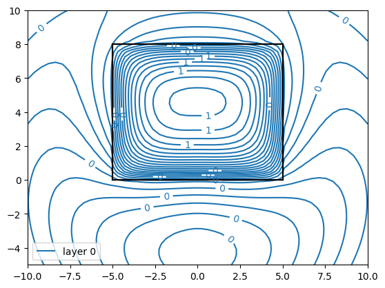
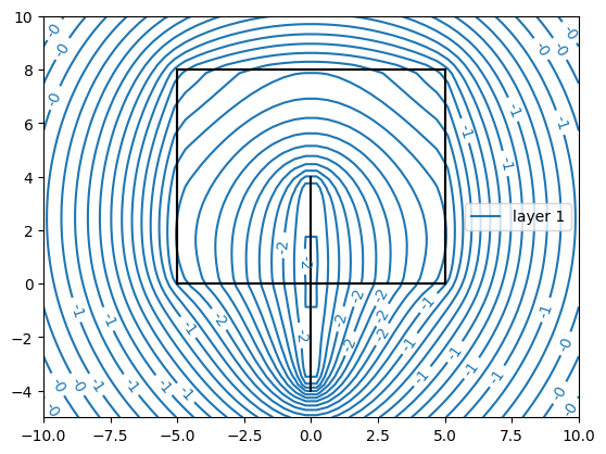
ls1 = tml.DitchString(ml, [(0, -4), (0, 0), (0, 4)], 100, order=3, layers=[1])
rf = tml.Constant(ml, xr=0, yr=-100, hr=2)
ml.solve()
ml.plots.contour([-10, 10, -5, 10], 50, [0], 30)
ml.plots.contour([-10, 10, -5, 10], 50, [1], 30)
Number of elements, Number of equations: 13 , 129
.
.
.
.
.
.
.
.
.
.
.
.
.

solution complete
[<matplotlib.contour.QuadContourSet at 0x7f8f2e861150>]
for ls in ls1.lslist:
    for i in range(ls.ncp):
        print(ml.head(ls.xc[i], ls.yc[i], ls.layers))
[-2.28658741]
[-2.28658741]
[-2.28658741]
[-2.28658741]
[-2.28658741]
[-2.28658741]
[-2.28658741]
[-2.28658741]
ml = tml.ModelMaq(kaq=[1, 2], z=[10, 5, 4, 0], c=20)
xy = [(-5, 0), (0, 0), (5, 0), (5, 8), (-5, 8)]
p1 = tml.PolygonInhomMaq(
    ml,
    xy=xy,
    kaq=[1, 2],
    z=[11, 10, 5, 4, 0],
    c=[2, 2],
    topboundary="semi",
    hstar=1.0,
    order=5,
    ndeg=2,
)
ls1 = tml.DitchString(ml, [(0, -4), (0, 0), (0, 4)], 100, order=3, layers=[1])
rf = tml.Constant(ml, xr=0, yr=-100, hr=2)
ml.solve()

ml.plots.contour([-10, 10, -5, 10], 51, [0], 30)
ml.plots.contour([-10, 10, -5, 10], 51, [1], 30)
Number of elements, Number of equations: 13 , 129
.
.
.
.
.
.
.
.
.
.
.
.
.

solution complete
[<matplotlib.contour.QuadContourSet at 0x7f8f2e982cd0>]